
Deep Q-Network -- Tips, Tricks, and Implementation
Q-Learning
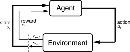
Q-learning is one of the fundamental methods of solving a reinforcement learning problem. In reinforcement learning problem, there is an agent that observes the present state of an environment, takes an action, receives a reward and the environment goes to a next state. This process is repeated until some termination criterion is met. The batch of state, action, and reward forms one trajectory of the environment. The goal of the agent is to maximize its total expected reward obtained in one trajectory. The following figure represents an archetypal setting of a reinforcement learning problem:
Q-learning solves a reinforcement learning problem by giving us the measure of goodness of actions at a given state. Assume that we are solving a reinforcement learning problem and the environment presents us the observation \(s'\). We can choose one of the two actions \(a_1\) or \(a_2\) at the presented state \(s'\). Assume that a fairy has given us access to a function \(Q(s, a)\) that can give us a measure of goodness of all actions \(a\) at any given state \(s\). We can check whether \(Q(s', a_1) > Q(s', a_2)\). If it is true, we will take action \(a_1\) and state \(s'\) otherwise we will take action \(a_2\).
Q-learning is all about finding the function \(Q(s, a)\) thats why it is called Q-learning.
How to find the function \(Q(s, a)\)?
To understand how to find the function \(Q(s, a)\), we first need to know what does \(Q(s, a)\) stands for. \(Q(s, a)\) represents the total maximum cumulative reward that we can get in the reinforcement learning problem after taking action \(a\) at state \(s\) until the end of the episode.
The following figure represents a portion of a trajectory in a reinforcement learning setting.

The above figure tells us that we are at state \(s_t\), we take action \(a_t\) and we reach to a new state \(s_{t + 1}\). As we know \(Q(s_t, a_t)\) represents the highest cumulative reward that we can get at state \(s_t\) after taking action \(a_t\). From the above figure, we see that after taking actions, \(a_t\) at state \(s_t\) we receive a reward \(r_t\) and we reach to a new state \(s_{t + 1}\). Note that the maximum reward that we can get at state \(s_{t + 1}\) is \(\max_{a_{t + 1}} Q(s_{t + 1}, a_{t + 1})\). Hence \(Q(s_t, a_t)\) must satisfy the following equation:
\[Q(s_t, a_t) = r_t + \max_{a_{t + 1}} Q(s_{t + 1}, a_{t + 1})\]However, we have just sampled one trajectory and based on just few samples, our estimate of the true Q-values may not be correct. So we will change the Q-values only little bit towards this new estimate. This little movement is determined by a constant called learning rate as shown in the following equation:
\[Q(s_t, a_t) \leftarrow \alpha_t (r_t + \max_{a_{t + 1}} Q(s_{t + 1}, a_{t + 1})) + (1 - \alpha_t) Q(s_t, a_t)\]where \(\alpha_t\) is the learning rate constant.
The trick to obtain \(Q(s, a)\) is to define \(Q(s, a)\) arbitrarily for all state and action pairs initially and then iteratively change \(Q(s, a)\) such that it satisfies or come close to satisfying the above equation for all states, actions pairs.
It is important to note here that it does not matter what policy is used to generate the trajectories as long as all states and actions are explored. The policy that is used to generate trajectories is generally referred as behavior policy. The policy for which we update the Q-values is called the target policy. In Q-learning, we collect the trajectories from some behavior policy and update the Q-values for the optimal policy. Since the behavior and target policy are not the same for Q-learning, Q-learning is an off-policy method. Although, Q-learning is an off-policy method, it makes sure that as long as the behavior policy is sufficiently exploratory i.e. the behavior policy ensures that all the state, action pairs would have non-zero probability of occurring, Q-learning would converge to the optimal policy for a finite state-action reinforcement learning problem.
Exploration policies
Mainly two type of exploration policies are used in \(Q\)-learning algorithms:
\(\epsilon-\)greedy policy: The epsilon greedy policy is defined as follows: 1) Toss a biased coin which can turn up to head with probability \(\epsilon\), 2) If the coin turn up to head then take a random actions 3) if the coin turn up to tail then take the action which has the highest \(Q\)-value at the given state.
Softmax (Boltzman) policy: The softmax policy choose action \(a\) at the given state \(s\) with the probability \(p(s, a)\) where \(p(s, a) = \frac{e^{Q(s, a) / T}}{\sum_b e^{Q(s, b) / T}}\) where \(T \in (0, \infty)\) is called temperature parameter.
Note that when \(T \rightarrow 0\), the Boltzman policy goes towards a greedy policy that always chooses the action with the maximum \(Q(s, a)\). When \(T \rightarrow \infty\), then policy converges towards a uniform policy that chooses all the actions with the uniform probability.
We need to choose the parameters for the exploration policies to ensure that we explore all the actions at a given states.
A classical example from grid world
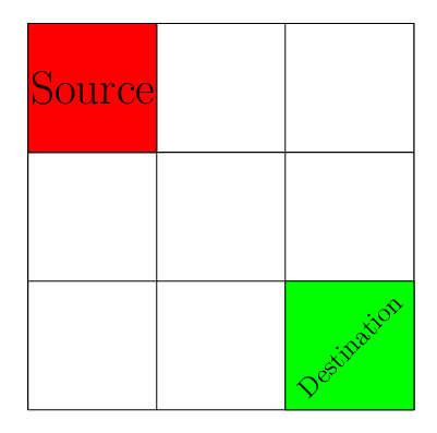
A classical problem where many Q-learning tutorial starts is the grid-world problem. The essence of this problem is in the following figure. There is a grid. You start with the source position. At each position, you can go the next position in the grid which is either up, down, right, or left of the present position. Your goal is to reach the destination position of the grid as quickly as possible.
Since our goal is to reach to the destination position from source as quickly as possible, we will define a reward mechanism that reflect this desired behavior in the agent. One easy way to do this is that we penalize each step taken by the agent with the reward of \(-1\). Therefore, to maximize her reward, the agent needs to reach to the destination as quickly as possible.
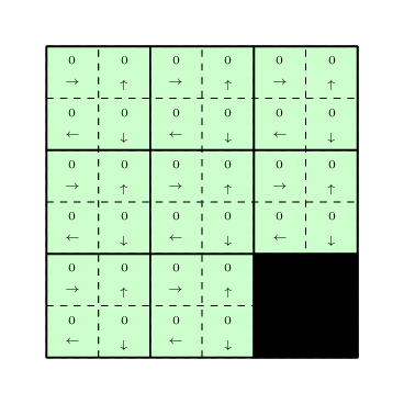
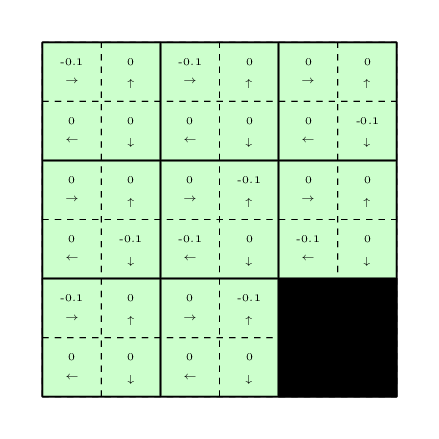
To use the Q-learning, we need to assign some initial Q-values to all state-action pairs. Let us assign all the Q-values to \(0\) for all the state-action pairs as can be seen in the following figure.
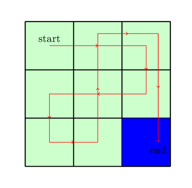
Lets use a Boltzman policy as the exploration policy for the problem with the temperature parameter \(1\). Since initially all the \(Q-\)values are equal, our exploration policy will choose a random actions at each state. It will keep choosing the random actions until it reaches to the destinations. Assume that it chooses the following path to reach to the destinations shown in the figure below.
After collecting this trajectory, we will update the \(Q-\)values using the \(Q-\)learning update equation:
\[Q(s_t, a_t) \leftarrow \alpha_t (r_t + \max_b Q(s_{t + 1}, b)) + (1 - \alpha_t) Q(s_t, a_t)\]The updated \(Q-\)values are shown below:
After doing the above procedure of collecting a trajectory and updating the \(Q-\)values multiple times, the final \(Q-\)values that we will achieve are the following:
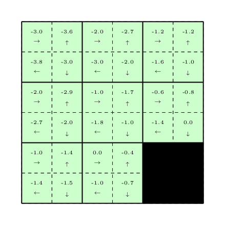
Knowing the above \(Q-\)values, we just need to choose the actions with the highest \(Q-\)values at each state to reach to the destination as soon as possible. The code for tabular Q-learning can be found here.
Problem of continuous state-space and the curse of dimensionality
Note that in the grid world problem, the state-space and action-space both are discrete which makes it easy to build a tabular representation of Q-values and keep updating it until convergence. However, continuous state-space makes Q-learning harder for following two reasons:
- We collect trajectories from the environment and based on the states that we visit in the trajectory, we update \(Q(s, a)\) for them. It is impossible to visit all the states when the states are continuous hence it is not feasible to build a tabular representation of \(Q(s, a)\) and updating it.
- Even if we decide to discretized the state-space to build a tabular representation, we need a lot of trajectories to find a good estimate of \(Q(s, a)\).
A Solution for continuous state-space
One solution for the continuous state-space problem is to use function approximation. The function approximation is a fancy way to say that we have a function \(f\), parametrized by \(w\), that gives us an approximation of true action-values \(Q(s, a)\). For example, we can use a neural network as following to approximate the action-values.
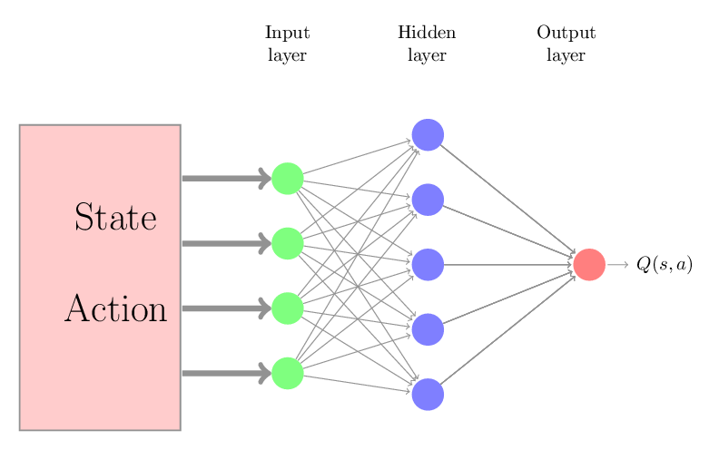
We can initialize parameters of neural networks (\(w\)) arbitrary and we can keep changing the \(w\) such that we minimize the following error
\[w = \arg\!\min\left(f^w(s, a) - \left(r + \max_b(f^w(s', b)\right) \right)^2\]Theoretical instability of Q-learning with function approximation
Q-learning is a bootstrapping method. By bootstrapping, we mean updating the action-values estimate on the basis of other action-values estimate. Off-policy bootstrap methods are known to diverge and can potentially give infinite Mean Square Error (MSE) on the optimization objective.
Deep Q-Network (DQN) to rescue
DQN approach is introduced to make Q-learning stable mainly for the high dimensional problems. DQN approach incorporates several techniques to make Q-learning stable that are enumerated as following:
Replay buffer
Q-learning with function approximation solves a regression problem where it moves the network parameters such that it reduces the TD-error. This is a supervised learning problem and supervised learning algorithms do good when the data comes from an independent-identical distribution (IID). But in a reinforcement learning problem, the states, actions, rewards tuples are sequential in nature. It is not a good idea to reduce the MSE on this sequential data. Moreover, in online Q-learning, once we used a data point to update the models, we don’t reuse it. Replay buffer is introduced to tackle these two problems. The idea behind replay buffer is simple and effective. Replay buffer stores the each interactions from the environment in the form of tuples of state, action, and rewards. It selects a batch of random data points from the history and use them for updating the Q-network parameter. We implemented a class for replay buffer. This class provides methods for adding the new experience and sampling a batch of random experiences from the buffer.
class ReplayBuffer(object):
    def __init__(self, buffer_size):
        self.buffer_size = buffer_size
        self.num_items = 0
        self.buffer = deque()

    def sample(self, batch_size):
        return random.sample(self.buffer, batch_size)

    def add(self, item):
        if self.num_items < self.buffer_size:
            self.buffer.append(item)
            self.num_items += 1
        else:
            self.buffer.popleft()
            self.buffer.append(item)

    def add_items(self, items):
        for item in items:
            self.add(item)

    def add_batch(self, batch):
        keys = ["states", "actions", "rewards", "next_states", "dones"]
        items = []
        for i in range(len(batch["states"])):
            item = []
            for key in keys:
                item.append(batch[key][i])
            items.append(item)
        self.add_items(items)

    def sample_batch(self, batch_size):
        keys = ["states", "actions", "rewards", "next_states", "dones"]
        samples = self.sample(batch_size)
        samples = zip(*samples)
        batch = {key: np.array(value) for key, value in zip(keys, samples)}
        return batch

    def count(self):
        return self.num_items
Target Network
Note that in Q-learning, we changes the weights of the network such that our network reduces the following TD error:
\[(f^w(s, a) - (r + \max_b f^w(s', b))^2\]This problem is minimizing the mean square error where our target is \(r + \max_b f^w(s', b)\). Note that the target of this minimization problem is changing in each iterations. Its like trying to hit a moving target. This is one of the main source of the instability of Q-learning. To overcome this problem, a clever idea is proposed by the original DQN paper. The idea is to choose a different network for choosing the action-values for the next states and change the parameters of this network slowly towards the parameters of the actual \(Q-\)network. The authors refer to this network as the target network. Assume that \(w\) and \(w'\) represent the weights of \(Q-\)network and target network respectively then we will change the \(w\) to minimize the following errors:
\[w = \arg\!\min\left(f^w(s, a) - \left(r + \max_b(f^{w'}(s', b)\right) \right)^2\]Their are two main strategies to update the parameters of the target networks (\(w'\)) – Hard update and Soft update.
Hard update rule was proposed in the orignal DQN paper. In this the target network weights are synchronized with the \(Q-\)network weights periodically after each \(N\) number of iterations. Essentially:
\[w' \leftarrow w \text{ when}\mod(n, N) = 0\]where \(n\) is the number of iterations.
Soft update rule was proposed in a subsequent paper where the authors used the tricks of DQN with actor-critic methods to solve reinforcement learning problems in continuous actions spaces. The soft update rule is in each iterations update the target network weights slowly with the Q-network weights.
\[w' \leftarrow \tau w + (1 - \tau) w' \text{ with } \tau \ll 1\]Both the soft and hard updates of the target network ensures that the targets of the Q-learning doesn’t change abruptly as we are updating the Q-network weights thus helps in stabilizing the learning.
To create a target network, I first defined a function q_network as shown below.
def q_network(states, observation_dim, num_actions):
    observation_dim = np.prod(observation_dim)
    x = states
    W1 = tf.get_variable("W1", [observation_dim, 20],
                         initializer=tf.contrib.layers.xavier_initializer())
    b1 = tf.get_variable("b1", [20],
                         initializer=tf.constant_initializer(0))
    z1 = tf.matmul(states, W1) + b1
    x = tf.nn.elu(z1)
    W2 = tf.get_variable("W2", [20, num_actions],
                         initializer=tf.contrib.layers.xavier_initializer())
    b2 = tf.get_variable("b2", [num_actions],
                          initializer=tf.constant_initializer(0))
    q = tf.matmul(x, W2) + b2
    return q
I called this function twice with different name scopes to create one set of weights for action-value network and the other set of weights for the target network.
with tf.variable_scope("q_network"):
    self.q_values = self.q_network(self.states, self.observation_dim, self.num_actions)
with tf.variable_scope("target_network"):
    self.target_q_values = self.q_network(self.next_states, self.observation_dim, self.num_actions)
To synchronize the weights between target network and action-value network, I first grab the variables of the target network and \(Q-\)network and then create ops for assigning the target variables with new-values. For example, following code creates the ops for the soft-target updates.
target_ops = []
q_network_variables = tf.get_collection(tf.GraphKeys.GLOBAL_VARIABLES, scope="q_network")
target_network_variables = tf.get_collection(tf.GraphKeys.GLOBAL_VARIABLES, scope="target_network")
for v_source, v_target in zip(q_network_variables, target_network_variables):
    target_op = v_target.assign_sub(self.target_update_rate * (v_target - v_source))
    target_ops.append(target_op)
self.target_update = tf.group(*target_ops)
Now updating the target network is running the ops with the tensorflow session.
Clipping the gradients and bounding the loss
Clipping the gradients
Even after applying the previous trick of target network, in some iterations the TD error in Q-learning can be large. This large TD-error will generate large gradients of parameters with respect to loss which can destabilize the whole learning.
To overcome this problem, we can borrow a trick from the exploding gradient problem in Recurrent Neural Network (RNN). The trick is simple, just clip the gradient such that the norm of the gradient stays within a certain threshold. This threshold is a hyper-parameter. One good heuristic for setting this hyperparameter is to look for the average norm of the gradients for sufficiently long updates. A value of the threshold between half to ten times of this average norm would usually allow convergence although the rate of convergence can vary.
Its easy to clip the gradients in tensorflow and apply the clipped gradients for updating the parameters. The following code provides an example of clipping and applying the gradients.
self.gradients = self.optimizer.compute_gradients(self.loss, var_list=self.trainable_variables)
self.clipped_gradients = [(tf.clip_by_norm(grad, self.max_grad_norm), var) for grad, var in self.gradients]
self.train_op = self.optimizer.apply_gradients(self.clipped_gradients, global_step=self.global_step)
Bounding the loss
Another way to stabilize the learning is by bounding the loss. Assume that we are solving a regression problem. Our prediction is \(\hat{y}\) and our target is \(y\). The error in this case is \(e = y - \hat{y}\). There are many ways to define the loss using the error. There are two common approaches: square-loss and absolute-loss.
There are some desirable properties in the square-loss that makes it apt for a regression problem. The gradient of the square-loss is directly proportional to the error. When the error is small, the update of the parameter will also be small. However, there is a flip side of this desirable property. When the error is big, there could be a huge change to the parameters. This could cause the instability in Q-learning.
On the other hand, the gradient of the absolute-loss is constant independent of the error. This has a very undesirable effect when the error is small. Even when the error is small, this can cause the significant change in the parameters and make it unsuitable for stochastic gradient based optimization method. However, the absolute loss has constant gradient even when the error is big so parameters will not change a lot when the error is big.
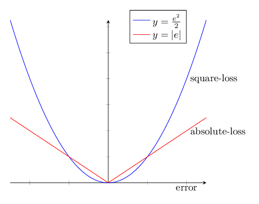

The summary from the above discussion is we have two ways to measure loss: square-loss and absolute-loss. Square-loss has the desire property when the error in the regression is relatively small and absolute-loss has the desire property when the error is relatively large. We can come up with a hybrid approach where we measure loss as a combination of square-loss and absolute-loss. This hybrid approach is called huber-loss. Huber loss is defined as follows:
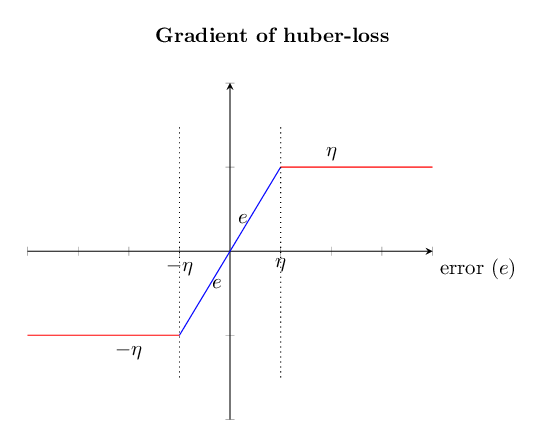
\[\text{huber-loss}(e) = \left\{\begin{array}{llr} &0.5 e^2 &\text{when } |e| < \eta\\ & \eta\left(|e| - 0.5 \eta\right) & \text{when } |e| \geq \eta \end{array}\right.\]where \(\eta\) is a hyper-parameter that we choose.
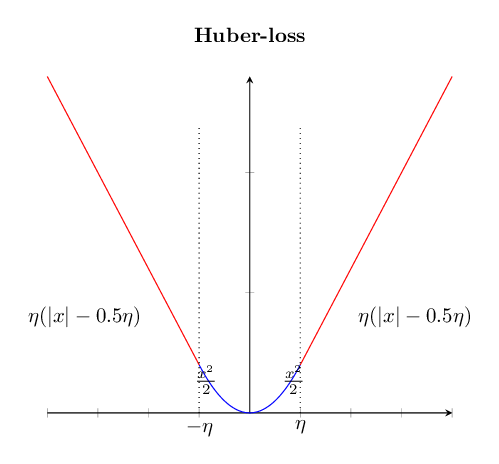
Note that the gradient for the huber-loss is bounded by \(\eta\) as is shown in the following figure.
The following code can serve as an example of implementing the huber loss in tensorflow.
error = self.action_scores - self.target_values
abs_loss = tf.abs(error)
square_loss = 0.5 * tf.pow(error, 2)
self.huber_loss = tf.where(abs_loss <= self.huber_loss_threshold,
                           square_loss,
                           self.huber_loss_threshold * (abs_loss - 0.5 * self.huber_loss_threshold))
Difference between bounding the loss and clipping the gradient
There is a subtle difference between bounding the loss using the huber-loss technique and clipping the gradient as explained below:
-
While clipping the gradients, we first compute the gradients of each trainable variables using back propagation then we clip the gradients and apply it to change the variables using the Stochastic Gradient Descent (SGD) method.
-
In bounding the loss, we change the loss function such that the gradient of the loss with respect to error will be bounded. Then this bounded gradient will be back-propagated in computing the gradients for all other trainable variables in the neural network architecture.
Using this comparison, we can say that clipping the gradient is a more aggressive way to not let the parameters change a lot in comparison to bounding the loss.
Applying DQN in continuous state-space problems
For this demo purpose, I chose the Cartpole environment to apply the DQN algorithm.
According to openai gym documentation, the cartpole problem is defined as following:
Cartpole: A pole is attached by an un-actuated joint to a cart, which moves along a frictionless track. The system is controlled by applying a force of \(+1\) or \(−1\) to the cart. The pendulum starts upright, and the goal is to prevent it from falling over. A reward of \(+1\) is provided for every timestep that the pole remains upright. The episode ends when the pole is more than 15 degrees from vertical, or the cart moves more than \(2.4\) units from the center.
Goal: We set our time horizon to \(200\) time steps. In our experience, we found out that \(200\) is a sufficiently big number to ensure that we found a good policy to balance the cartpole for ever. Our goal is to create an agent that can keep the Cartpole stable for the \(200\) time-steps using the DQN algorithm. The maximum reward that we can obtained in this environment is \(200\).
Results
The following figure shows the progress of our approach as the number of iterations:
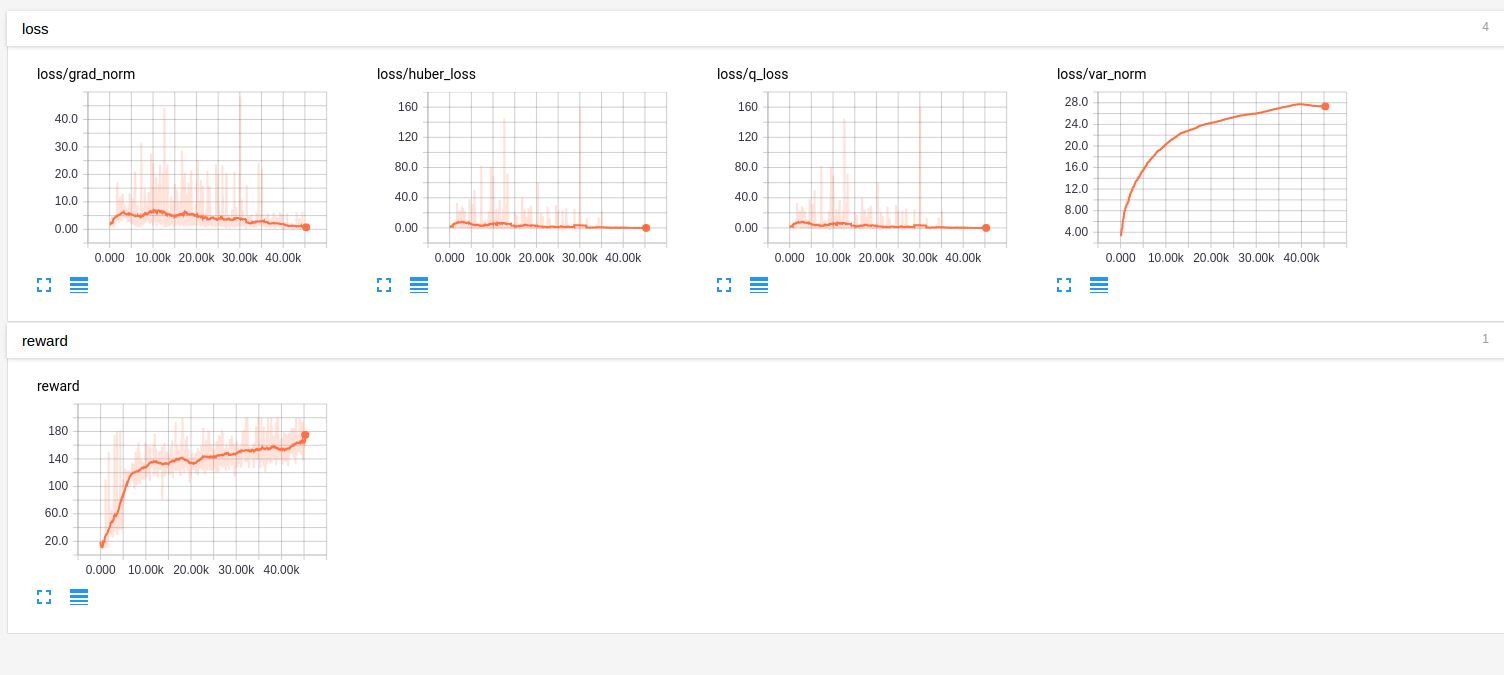
You can see that DQN approach is able to find a good policy for cartpole environment.
Concluding Remarks:
DQN algorithm solves the instability issues in Q-learning by applying the following tricks:
- Target Network
- Replay buffer
- gradient (loss) clipping
We see that DQN algorithm can be trained to learn a good policy for a continuous state-space problem. The full code for this problem can be found here