Motivation

Ever since I started working on reinforcement learning (RL), specially policy gradient algorithms, one thing always annoyed me was that we need a simulator to generate trajectories from a policy. We need these trajectories to improve our policy using policy gradient theorem. Many times we do not have a simulator to generate trajectories, we just had some past data. To use reinforcement learning, we first need to create a simulator using supervised learning and then generate trajectories using this simulator. However, there is a problem here. The created simulator has some inherent sample biasness and it will also have some fitting error. Then we use the reinforcement learning to find a policy using this simulator. We have to tackle three kinds of error in this approach:

1. Sampling error
2. Supervised learning error
3. Reinforcement Learning error

In this blog, we will know an approach where we don’t need to fit a supervised learning model on the data. We can directly use the past data to train a policy. This approach is known as Path Consistency Learning. It was published in a recent article by Google Brain team.

What is Path Consistency Learning?

As is hinted in the name of the algorithm, there should be some consistency criterion that the optimal policy should satisfy. We will use the collected trajectories to change the parameters of policy until the consistency criterion is not satisfied. In the process, we will get the optimal policy.

What is this consistency criterion?

To understand the consistency criterion, look at the following figure.

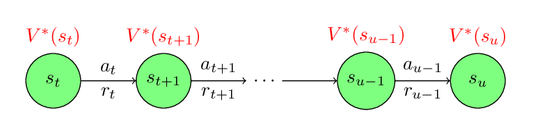
Assume that we collected a trajectory and in one portion of the trajectory we see the above transitions. Assume that \(\pi^{*}(\cdot|s)\) is the optimal policy and \(V^{*}(s)\) is the value function of the optimal policy then the Path Consistency criterion says that \(\pi^{*}(s)\) and \(V^{*}(s)\) must satisfy the following equation:

\[-V^*(s_t) - \sum_{t'=t}^{u-1} \gamma^{t'-t}\log\pi^*(a_{t'}|s_{t'}) + \sum_{t'=t}^{u-1} \gamma^{t'-t}r_{t'} + \gamma^{u-t} V^*(s_u) = 0\]

Note that the above condition must be satisfied by the optimal policy and optimal value function for all transitions. It does not matter that what policies are used to collect the transitions. We just need to keep changing our policy until it satisfy the consistency criterion. Once we find the policy that satisfy the consistency for all possible transitions, we can be sure that we find the optimal policy.

Proof [Math heavy]

To understand the proof of the consistency criterion, look at the following figure. Assume that we are at state \(s_0\). We can take action from the set \(\{a_1, a_2, \cdots, a_n\}\). If we take action \(a_i\) we get a reward \(r_i\) and we transition to the new state \(s_i\) where \(i \in \{1, 2, \cdots, n\}\). Assume that we already know the optimal future rewards from state \(s_i\) that is \(V^*(s_i)\) for \(i \in \{1, 2, \cdots, n\}\).

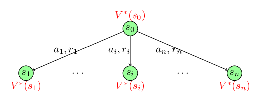
Our goal is to find the policy that maximizes our total reward at state \(s_0\). Assume that the optimal policy is \(\pi^*(s)\) that tells us the probability of choosing actions at state \(s\). Further, lets consider that according to the optimal policy \(\pi^*(s_0)\), we should choose actions \(\{a_1, a_2, \cdots, a_n\}\) with probability \(\{p_1^*, p_2^*, \cdots, p_n^*\}\) respectively. The total reward that we will obtain using the policy \(\pi^*(s)\) is

\[V^*(s_0) = \sum_{i=1}^n p^*_i(r_i + \gamma V^*(s_i)) - \tau \sum_{i=1}^n p^*_i \log p^*_i\]

Note that there is an extra entropy term on the right side of the equation. You can learn more about the use of entropy with policy gradient algorithm in our previous blog.

Using some algebra, we can write the above equation as

\[\begin{eqnarray} V^*(s_0) &=& -\tau\sum_{i=1}^n p^*_i \log\frac{p^*}{e^{(r_i + \gamma V^*(s_i))/\tau}}\\ &=& -\tau\sum_{i=1}^n p^*_i \log\frac{p^*_i}{\frac{e^{(r_i + \gamma V^*(s_i))/\tau}}{\sum_{j=1}^n e^{(r_j + \gamma V^*(s_j))/\tau}}} + \tau \log\sum_{j=1}^n e^{(r_j + \gamma V^*(s_j))/\tau} \end{eqnarray}\]

Note that the first term in the above equation is the KL-distance between two probability distribution: \(p_i^*\) and \(\frac{e^{(r_i + V^*(s_i))/\tau}}{\sum_{j=1}^n e^{(r_j + V^*(s_j))/\tau}}\). As we know the minimum value of KL-distance can be zero and \(V^*(s_0)\) is the maximum value for any probability distribution, we get the following identity:

\[\begin{eqnarray} p_i^*& = & \frac{e^{(r_i + \gamma V^*(s_i))/\tau}}{\sum_{j=1}^n e^{(r_j + \gamma V^*(s_j))/\tau}}\\ V^*(s_0) &=& \tau \log \sum_{j=1}^n e^{(r_j + \gamma V^*(s_j))/\tau} \end{eqnarray}\]

We can combine the above two equations, and can write

\[p_i^* = \frac{e^{(r_i +\gamma V^*(s_i))/\tau}}{e^{V^*(s_0)/\tau}}\]

Taking \(\log\) on both side of the equations, we get

\[-V^*(s_0) - \tau \log p_i^* + r_i + \gamma V^*(s_i) = 0 \;\;\forall\;\; i \in \{1, 2, \cdots, n\}\]

By recursively writing the equation for next states (\(V^*(s_i)\)) until the desired time step, we get the path consistency equation. \(\blacksquare\)

Using Path Consistency Learning to solve a reinforcement learning problem when we have access to off-policy data

The approach is similar to the way we use policy gradient algorithm. Lets assume that the policy is \(\pi_\theta(\cdot|s)\) that is parameterized by parameter \(\theta\), and the value function \(V_w(s)\) is parameterized by parameter \(w\). We get a portion of trajectory from off-policy data. Consider that the portion is \(\{(s_0, a_0, r_0), (s_{1}, a_{1}, r_{1}), \cdots, (s_N, a_N, r_N)\}\). We will compute the path consistency loss for the present policy as the following:

\[C(\theta, w) = \left(-V_w(s_0) - \sum_{t=0}^{N} \gamma^{t}\log\pi_\theta(a_{t}|s_{t}) + \sum_{t=0}^{N-1} \gamma^{t}r_{t} + \gamma^{N} V_w(s_N)\right)^2\]

We will keep changing \(\theta\) and \(w\), until we minimize this loss.

Path Consistency Learning to solve a classical control problem

For this demo purpose, I chose the Cartpole environment to apply the Path Consistency Learning algorithm.

According to openai gym documentation, the cartpole problem is defined as following:

Cartpole: A pole is attached by an un-actuated joint to a cart, which moves along a frictionless track. The system is controlled by applying a force of \(+1\) or \(−1\) to the cart. The pendulum starts upright, and the goal is to prevent it from falling over. A reward of \(+1\) is provided for every timestep that the pole remains upright. The episode ends when the pole is more than 15 degrees from vertical, or the cart moves more than \(2.4\) units from the center.

Goal: We set our time horizon to \(200\) time steps. In our experience, we found out that \(200\) is a sufficiently big number to ensure that we found a good policy to balance the cartpole for ever. Our goal is to create an agent that can keep the Cartpole stable for the \(200\) time-steps using the PCL algorithm. The maximum reward that we can obtained in this environment is \(200\).

Results

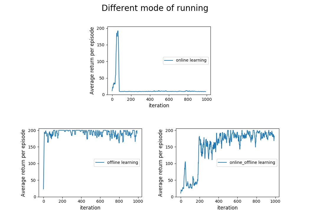
I experiment with three modes of learning. For the lack of better words, I named them as following:

1. Online Learning: In online learning, all the trajectories were generated using the interactions of the current polciy parameters with the environment and an update was made based only using these collected trajectories.
2. Online-Offline Learning: In online-offline learning, an agent collects one trajectory from the environment, make an update of the policy parameters using this trajectory and put this trajectory into an replay buffer. Subsequently, she samples \(20\) trajectories from the replay buffer and further use these trajectories to update the policy parameters. The sampling criterion is not uniform. If a trajectory has high total rewards, then it will have higher chances of being sampled.
3. Offline Learning: In offline learning, the agent just samples the trajectory from the replay buffer and use them to update the present policy parameters. I am using the replay buffer created during the online-offline learning mode. The sampling criterion in offline learningis same as in online-offline learning.