Policy Gradient

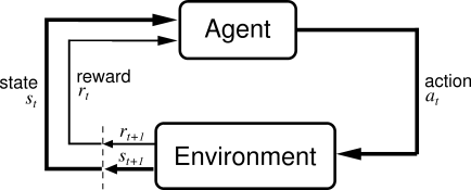
Policy gradient is a popular method to solve a reinforcement learning problem. In a reinforcement learning problem, there is an agent that observes the present state of the environment, takes an action according to her policy, receives a reward and the environment goes to a next state. This process is repeated until some terminating criterion is met. The sequence of state, action, and rewards forms one trajectory of the environment. The goal of the agent is to maximize its total cumulative reward obtained in one trajectory. The following figure represents an archetypical setting of a reinforcement learning problem:

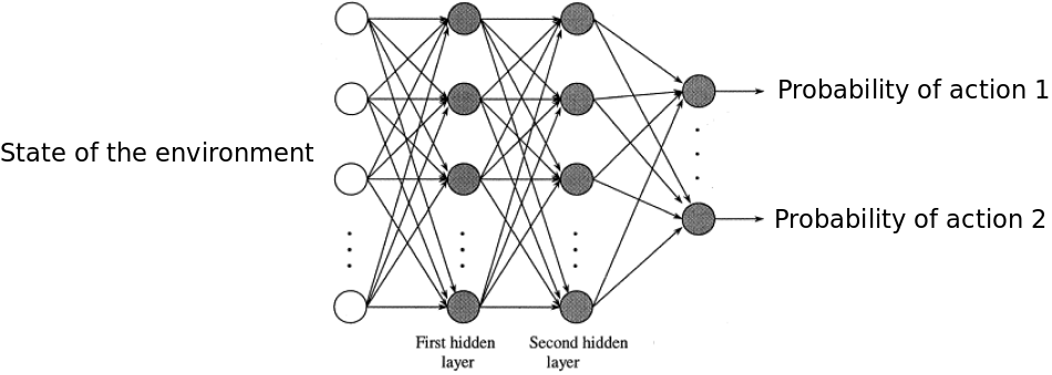
Policy gradient methods provide a way to solve a reinforcement learning problem. A policy is simply a function which takes the state of the environment as the input and gives the actions’ probabilities as the output. Usually, we use a parameterized policy and use a feed forward neural network to represent this policy. A typical policy network for a problem with discrete action space looks as the following:

To train a policy network, we initialize the parameters of the policy randomly and then apply the following steps until convergence:

1. collect a batch of trajectories by taking actions according to the policy
2. update the parameters using the whole batch.

Markovian Assumption of the policy gradient

Policy gradient algorithms are based on the assumption that the the only information that the policy need to know to take the optimal action is the present state. It does not matter how the present state is reached. This assumption is known as Markovian Assumption. However, this assumption may not be valid for all problems. For example, this assumption is not valid when creating an agent that can play the Pong game.

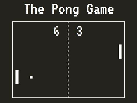
In the pong game, the environment provides the present state of the game that can be an image as above. By looking at the image, an agent cannot know the direction and speed of the ball, consequently the present state is not sufficient for the agent to determine her action. However, the agent can determine the speed and direction of the ball if she would have access to the past few frames along with the present frames. Precisely this trick was used by DeepMind in their seminal work. They stacked four images and passed it to a feed forward neural network that finally give them the action to take for their agent. However, this is an heurestic. It is not always possible to know how many past states are required to form an appropriate representation of the environment’s state for all the problems.

To go around this issue, in this blog we will use an approach based on Recurrent Neural Network. This idea is inspired by this work where the authors showed the efficacy of RNN in solving Partially-Observable MDPs.

Recurrent Neural Network for help in non-markovian setting

Recurrent Neural Networks (RNN) are very popular in machine learning when one has to deal with sequential data. RNNs have an internal state. This state keeps a representation of what has happened in the past. Then based on the present input and present state of the RNN, it decides the optimal output. Inspired by this, we used RNN to deal with non-markovian environment. Mainly, we used RNNs to parametrize the policy.

RNN for representing a policy

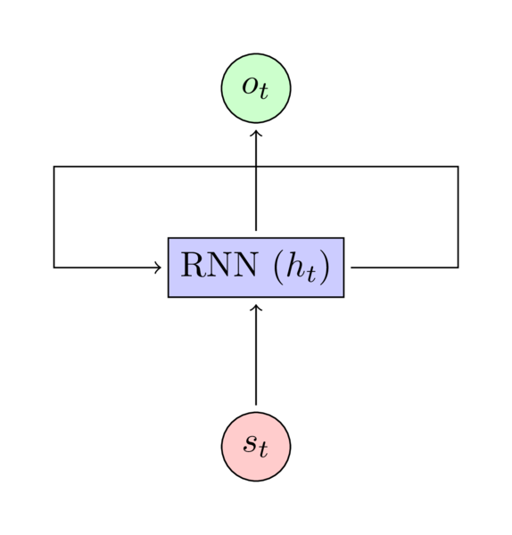
The input \(s_t\) to the above RNN is the observation from the environment. The \(h_t\) is representing the internal state of the RNN and \(o_t\) is the output that is in our case is the probability of all actions that we can take.

A trajectory

A trajectory is a set of tuples consisting of environment states, actions taken by the agent, and rewards starting from time \(t=0\) until some terminating criterion is met. Lets assume that when an environment is at state \(s_0\) at time \(t=0\), we take action \(a_0\), and receive reward \(r_0\). The environment goes to a new state \(s_1\) at which we take action \(a_1\) and receive reward \(r_1\) and so on. Assume that the environment meets some stopping criteron after time \(T\). This stopping criterion can be as simple as maximum \(T\) timesteps are allowed from the environment. The trajectory is \(\left\{(s_0, a_0, r_0), (s_1, a_1, r_1), \cdots, (s_{T-1}, a_{T-1}, r_{T-1}) \right\}\)

A trajectory using an RNN policy

In an RNN policy, RNN also has an internal state. This internal state changes as the environment state changes. When we use an RNN policy to generate actions, these internal states of RNN also become a part of trajectories. So we will have trajectories consisting of set of four tuples instead of the previous three tuples. The trajectory becomes \(\left\{(s_0, h_0, a_0, r_0), (s_1, h_1, a_1, r_1), \cdots, (s_{T-1}, h_{T-1}, a_{T-1}, r_{T-1})\right\}\) where \(h_t\) is the internal state of the RNN at time \(t\).

The code for collecting the trajectories for an rnn policy is as following:

    def collect_one_episode(self, render=False):
        states, actions, rewards, dones = [], [], [], []
        init_states = tuple([] for _ in range(self.num_layers))
        state = self.env.reset()
        init_state = tuple(
             [np.zeros((1, self.gru_unit_size)) for _ in range(self.num_layers)])
        for t in range(self.max_step):
            if render:
                self.env.render()
            state = self.preprocessing(state)
            action, final_state = self.policy.sampleAction(
                                        state[np.newaxis, np.newaxis, :],
                                        init_state)
            next_state, reward, done, _ = self.env.step(action)
            # appending the experience
            states.append(state)
            actions.append(action)
            rewards.append(reward)
            [init_states[i].append(init_state[i][0]) for i in
                                           range(self.num_layers)]
            dones.append(done)
            # going to next state
            state = next_state
            init_state = final_state
            if done:
                break
        returns = self.compute_monte_carlo_returns(rewards)
        returns = (returns - np.mean(returns)) / (np.std(returns) + 1e-8)
        episode = dict(
                    states = np.array(states),
                    actions = np.array(actions),
                    rewards = np.array(rewards),
                    monte_carlo_returns = np.array(returns),
                    init_states = tuple(np.array(init_states[i])
                                   for i in range(self.num_layers)),
                    )
        return self.expand_episode(episode)

Creating a batch from a trajectory

When we train an RNN, we pass it a batch of examples to update the parameters. Each example is a sequence of inputs. The length of this sequence is a hyper-parameter that we choose based on our understandings of the time dependencies in the sequence. To feed our trajectory for updating the RNN parameters, we need to convert our trajectroy into a batch of sequence. For example, for a batch of sequece of length \(4\), our trajectory will be transformed to something like the following:

Note that only the first RNN state of each sequence was stored in the batched sequence because for computing the loss only the first RNN state is required as will be clearer in the next section.

The following code does exactly as the above:

def expand_episode(self, episode):
        episode_size = len(episode["rewards"])
        if episode_size % self.num_step:
            batch_from_episode = (episode_size // self.num_step + 1)
        else:
            batch_from_episode = (episode_size // self.num_step)

        extra_length = batch_from_episode * self.num_step - episode_size
        last_batch_size = episode_size - (batch_from_episode - 1) * self.num_step

        batched_episode = {}
        for key, value in episode.items():
            if key == "init_states":
                truncated_value = tuple(value[i][::self.num_step] for i in
                                        range(self.num_layers))
                batched_episode[key] = truncated_value
            else:
                expanded_value = np.concatenate([value, np.zeros((extra_length,) +
                                                     value.shape[1:])])
                batched_episode[key] = expanded_value.reshape((-1, self.num_step) +
                                                         value.shape[1:])

        seq_len = [self.num_step] * (batch_from_episode - 1) + [last_batch_size]
        batched_episode["seq_len"] = np.array(seq_len)
        return batched_episode

Note that the trajectory length cannot always be multiple of the sequence length that we choose to train the RNN. To overcome this we will insert some dummy inputs in the last example as is done in the above code snippet.

Feeding the batched trajectory to compute loss in RNN based policy

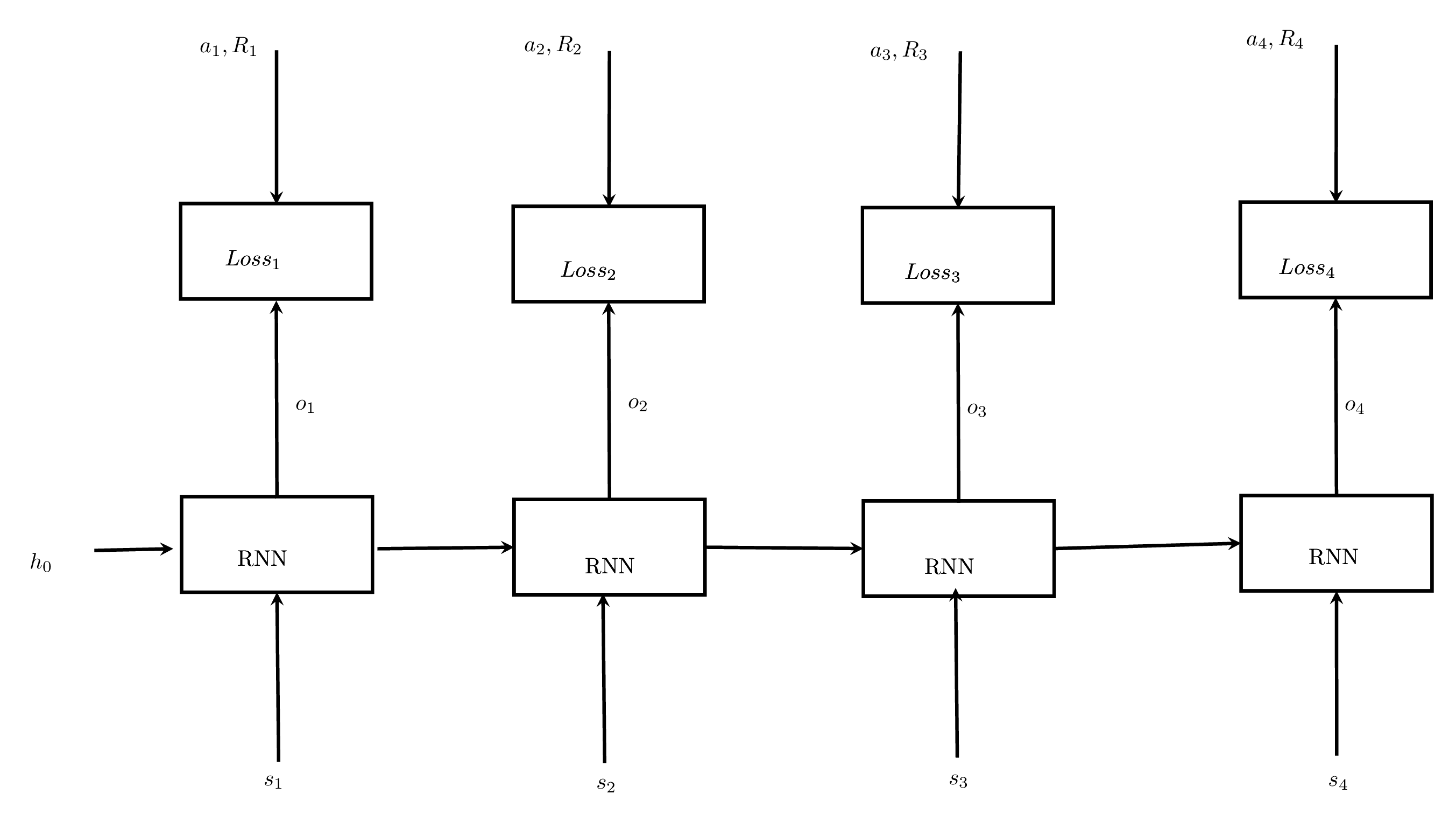
We feed a batch of sequence in the RNN. We just need to feed the first RNN state to compute the forward propagation. At each step, RNN computes the probability of taking all actions at the state that was fed to it. We see in the trajectory the actual action that was taken at that state then we compute the Policy Gradient Loss.

where \(o_i\) is the output of the RNN that represent the probability of all actions at state \(s_i\).

The following figure demonstrates the process of computing the loss.

Note that some of the states are dummy states in the batch and we don’t want to use the loss by them so we will use a sequence masking technique to make the contribution of their losses zero.

The follwoing 15 lines code in tensorflow takes care for us doing all the heavy lifting of computing the loss and updating the parameters.

  def create_variables_for_optimization(self):
    with tf.name_scope("optimization"):
      with tf.name_scope("masker"):
          self.mask = tf.sequence_mask(self.seq_len, self.num_step)
          self.mask = tf.reshape(tf.cast(self.mask, tf.float32), (-1,))
      self.pl_loss = tf.nn.sparse_softmax_cross_entropy_with_logits(
                                            logits=self.logit,
                                            labels=self.actions_flatten)

      self.pl_loss = tf.multiply(self.pl_loss, self.mask)
      self.pl_loss = tf.reduce_mean(tf.multiply(self.pl_loss, self.returns_flatten))
      self.entropy = tf.multiply(self.entropy, self.mask)
      self.entropy = tf.reduce_mean(self.entropy)
      self.loss = self.pl_loss - self.entropy_bonus * self.entropy
      self.trainable_variables = tf.get_collection(tf.GraphKeys.GLOBAL_VARIABLES, scope="policy_network")
      self.gradients = self.optimizer.compute_gradients(self.loss, var_list=self.trainable_variables)
      self.clipped_gradients = [(tf.clip_by_norm(grad, self.max_gradient), var)
                                  for grad, var in self.gradients]
      self.train_op = self.optimizer.apply_gradients(self.clipped_gradients,
                                                     self.global_step)

Solving a reinforcement learning problem with an RNN policy

To illustrate the application of a policy gradient algorithm to solve a reinforcement learning problem, we used the classical control problem called Acrobot. According to openai gym documentation, the acrobot problem is defined as follows:

The acrobot system includes two joints and two links, where the joint between the two links is actuated. Initially, the links are hanging downwards, and the goal is to swing the end of the lower link up to a given height.

Although Acrobot still satisfies the Markovian assumption, we will show that our RNN policy is able to learn a reasonably good policy for the Acrobot environment.

Goal: Our goal is to bring the Acrobot to a certain height as quickly as possible.

Results

The following figure shows the progress of our approach as the number of iterations:

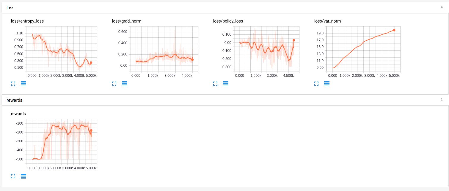
You can see that our approach is able to bring the Acrobot to a ceratin height in approximately 100 steps.

Concluding Remarks

Recurrent Neural Network can be used to solve RL problem when the Markovian assumptions are not valid. In our upcoming blogs, we will show how this RNN policy, equipped with few more tricks, can efficiently solve Atari games.