Multi-arm Bandit problem

Multi-arm bandit is a colorful name for a problem we daily face in our lives given choices. The problem is how to choose given multitude of options. Lets make the problem concrete. Assume that its Friday evening and you are planning to go to a fancy restaurant. Should you try your favorite restaurant or try some new restaurant. If you go for your favorite restaurant then you are exploiting your past knowledge and if you go for a new restaurant, then you are exploring which may be useful in future to find a better restaurant than your present restaurant. Unfortunately, it is also possible that you may come across some very bad restaurants during this exploration. The main question is how to balance the tradeoff between exploration and exploitation. Thompson Sampling essentially provides a way to solve this problem.

Thompson Sampling

Assume that there are two restaurants \(A\) and \(B\). Assume that restaurant \(A\) on an average \(\theta_1\) times align to your taste and restaurant \(B\) on an average \(\theta_2\) times align to your taste. In other words, if you go to restaurant \(A\), \(N\) times, then you will like the experience \(\theta_1 N\) times and if you go to restaurants \(B\), \(N\) times, then you will like the experience \(\theta_2 N\) times where \(\theta_1\) and \(\theta_2\) are some numbers between \(0\) and \(1\). Unfortunately these numbers \(\theta_1\) and \(\theta_2\) are unknown to you so you cannot know which restaurant you should choose. You go to restaurant very often and you want to maximize your chances of having good experiences in the restaurants during your life time. How should you choose these restaurants based on your experiences so far? Thompson Sampling comes to rescue here.

The idea behind Thompson Sampling is inspired by Bayesian Inference. Lets try to present the main idea behind Thompson Sampling as succinctly as possible below:

1. Lets assume that we have priors on unknown parameters that affects the reward for our bandit problem. In our restaurant example, the parameters are \(\theta_1\) and \(\theta_2\). The reward for bandit problem is essentially \(\theta_1\) and \(\theta_2\) which are the measure of goodness of the restaurant.
2. We sample a value of unknown parameters from this prior distribution.
3. We compute the reward from these sampled parameters.
4. We choose the actions which gives the highest reward.
5. We observe the actual reward gathered by taking our action.
6. We update the priors on the parameters using the observed reward.
7. We repeat the above procedure using the new posterior distribution.

Thompson Sampling in action

Now lets apply the Thompson Sampling to our restaurant hunting problem and see how does it help us in resolving the problem.

1. Since we don’t know anything about the restaurants initially, we can assume that the \(\theta_1\) and \(\theta_2\) parameters are uniformly distributed between \(0\) and \(1\). Note that we can also write a uniform distribution between \(0\) and \(1\) as a beta-distribution \(B(1, 1)\). Please read more about the beta-distribution here which is going to be helpful in understanding the upcoming text.

2. We sample a value for \(\theta_1\) and a value for \(\theta_2\) from their prior distribution. We choose the restaurant having the higher \(\theta\) values.

3. Assume that you chose the restaurant \(A\) in the previous step. You go to the restaurant and if you have the good experience in the restaurant, you give it \(+1\) reward otherwise you would give it a \(0\) reward.

4. Now we need to update the distribution for \(\theta_1\) based on the reward that we observed in the previous step. Since our prior distribution was the beta-distribution, it is easy to do as described below:

   If your prior distribution for \(\theta_1\) is \(B(\alpha, \beta)\) you receive the reward \(r\) for going to restaurant \(A\) then the posterior probability distribution for \(\theta_1\) is \(B(\alpha + r, \beta + (1 -r))\).

5. Now to choose a restaurant second time, you sample new values for \(\theta_1\) and \(\theta_2\) but you use the updated probability distribution for the restaurant \(A\) that was chosen in the first trial and you keep going on like that to choose restaurants.

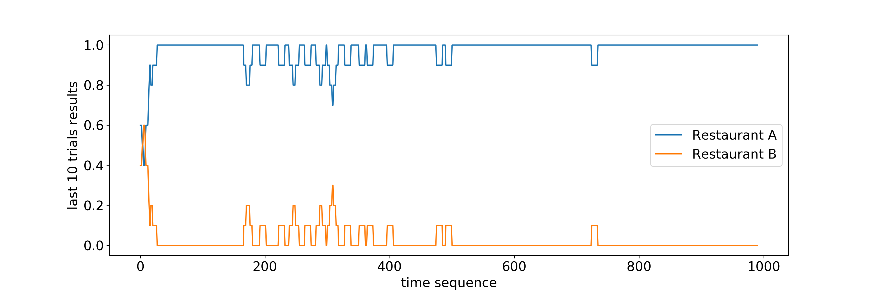
Now lets see how does Thompson Sampling helps us in finding the best restaurant. We will simulate this behavior. For this simulation, we will assume that the true value of \(\theta_1\) is \(0.9\) and true value of \(\theta_2\) is \(0.7\). We would like to see that as time progress, Thompson Sampling would recommend us restaurant \(A\) more and more.

In the following figure, we plot how Thompson sampling chooses between restaurant \(A\) and restaurant \(B\). Each point is telling us the fraction of time restaurant \(A\) and restaurant \(B\) were chosen by Thompson sampling in the previous \(10\) trials. It is interesting to see that in this case Thompson sampling figures out pretty quickly (approximately \(10\) trials) that it should stick with restaurant \(A\) for better experience.

It is interesting to note that Thompson Sampling is doing a good job in finding the best restaurant when we have to find the best restaurants only among two restaurants. An obvious question comes, is Thompson Sampling easily extendable. In other words, can it gives us a similar performance when we had to find the best restaurant among \(N\) restaurants where \(N > 2\). To investigate this question, we did a simulation as you can see in the following figure.

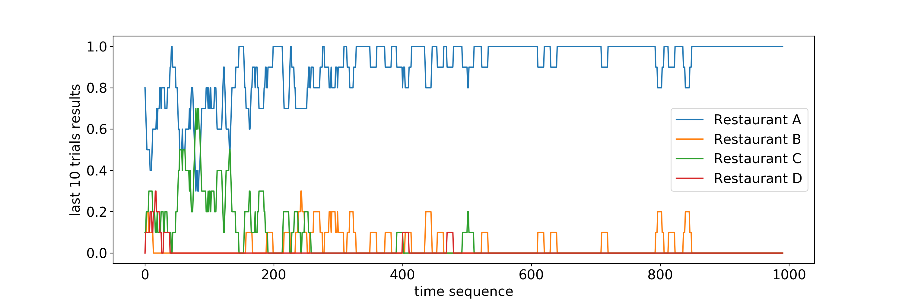
For the above simulation, we assume that the true thetas parameter of Thompson Sampling are \(0.95, 0.9, 0.85\) and \(0.8\) for restaurant A, B, C, and D respectively. As you can see in the above figure, Thompson Sampling is able to recommend the best restaurant \(A\) consistently although it is taking approximately \(200\) trials for Thompson Sampling to consistently make this claim.

At this juncture of this blog, we can ask some important questions as following:

1. Can we change Thompson Sampling somehow to increase the convergence speed of Thompson Sampling?
2. Can we utilize some side information (such as recipe of the restaurants, information about chefs etc) to decrease the learning time for Thompson Sampling?

Contextual Thompson Sampling is precisely the answer of the above questions that will be the focus of the rest of the blog.

Contextual Thompson Sampling

Following the previous case (Simple Thompson Sampling), we will first use a mathematical abstraction to explain Contextual Thompson Sampling. Further, we will elaborate this concept with the help of our ongoing restaurant search problem.

As is suggested in the name, in Contextual Thompson Sampling there is a context that we will use to select arms in a multi-arm bandit problem. The context vector encapsulates all the side information that we think can be useful for determining the best arm. Lets denote a context vector by the symbol \(x\). For each arm, we want to determine a set of parameters \(\theta\) that can tell us how to choose an arm given a context. We will assume that we also know a function \(f\) that tells us the relationship between parameter vector \(\theta\), context vector \(x\), and expected reward \(r\) of the arm. In essence,

\[\mathbb{E}[r(x)] = f(x; \theta)\]

You may say that it is difficult to know the function \(f\) but we can always choose \(f\) to be a high capacity neural network model that can model even very complex relationship between \(x\) and \(\theta\). Although training time of such a high capacity neural network model can be long because it would require lot of data.

The training process of Contextual Thompson Sampling is similar to Simple Thompson Sampling.

1. At time \(t=0\), we observe a context \(x_0\).
2. For each arm \(a\), we assume that \(\theta_a\) is distributed according to the probability distribution \(D(\alpha_a)\) where \(\alpha_a\) are the parameters of the distribution.
3. For each arm, we will start with some initial value of \(\alpha_a\). Lets call this initial value \(\alpha_a(0)\).
4. We will sample \(\theta_a\) according to the distribution \(D(\alpha_a(0))\) for each arm \(a\).
5. We will compute the expected reward \(f(x_0, \theta_a)\) for each arm.
6. We choose the arm that has the maximum value of \(f(x_0, \theta_a)\)
7. We observe the actual reward \(r_0\) for playing this arm.
8. We repeat the above process \(N\) times.
9. Subsequently, we update the parameters \(\alpha_a\) for each arm using the maximum likelihood estimator of \(\alpha_a\) after observing the reward \(r\).
10. We keep repeating the above process until some predefined convergence criterion is met.

Contextual Thompson Sampling for Restaurant Searching Problem

Lets first consider the context vector. Assume that the context vector consists of following elements: day of the week, and weather. Consider the following property of each of the context field:

1. Day of week: This feature represents the day that we visit the restaurant. We are assuming that if there is some impact of day of week on us liking the restaurant that Thompson Sampling will be successfully able to capture this impact.

2. Weather: This feature represents the weather we visit the restaurant. Assume that this field can be of one of two types: hot weather or cold weather.

Now lets make the most important assumption. Assume that we like restaurant \(A\) when the weather is hot and we like restaurant \(B\) when weather is cold. In other words, only the weather field in the context vector that gives us the significant information about us liking a restaurant.

In Thompson Sampling, the context vector consists of day of week and weather. We use the one-hot encoded representation to represent this context vector. So our context vector for the restaurant search problem is \(9\) dimensional vector. The first seven dimension out of these \(9\) dimensions represent day of week. The next \(2\) dimension represent the weather. For example, if the context vector is \([1, 0, 0, 0, 0, 0, 0, 1, 0]\), then it implies that we are visiting the restaurant in a hot day where day of week is Monday.

We further assume that the expected reward of a restaurant is a linear function of context vector and the restaurant parameters (\(\theta_A\) and \(\theta_B\)). In mathematical terms,

\[\begin{eqnarray} E[r_A] &=& \theta_A^Tx \\ E[r_B] &=& \theta_B^Tx \end{eqnarray}\]

We further assume that initial distribution of parameters \(\theta_A\) and \(\theta_B\) for restaurant \(A\) and restaurant \(B\) are normally distributed with \(\mathcal{N}(\mu_A(0), \Sigma_A^2(0)\mathcal{I})\) and \(\mathcal{N}(\mu_B(0), \Sigma_B^2(0)\mathcal{I})\) respectively. Now our goal is to find the posterior distribution for \(\theta_A\) and \(\theta_B\) after looking at our observations. Fortunately, it is easy to do with the help of Laplace Approximation. In short, we are applying the Bayesian Logistic Regression in a sequence. This is a good tutorial on Laplace Approximation.

But in short, the result are as following:

1. Assume that we visited restaurant \(A\), \(n\) times.
2. The context for these \(n\) times was \(x_1, x_2, \cdots, x_n\) which is a \(9\) dimensional vector.
3. Our experience at these \(n\) times is denoted by \(y_1, y_2, \cdots, y_n\) which is a binary number \(0\) or \(1\).
4. The formula to update the mean parameter \(\mu_A(0)\) for restaurant \(A\) is \(\mu_A(1) = \arg\!\max_{w} \sum_{i=1}^n\left(\text{sigmoid}((2 * y - 1) w^T x_i)) - \frac{1}{2}(w - \mu_A(0))^T \Sigma_A(0)^{-1} (w - \mu_A(0))\right)\)
5. The formula to update the variance parameter \(\Sigma_A(0)\) is as following \(\Sigma_A^{-1}(1) = \Sigma_A^{-1}(0) + \sum_{i=1}^N \text{sigmoid}((2 * y - 1) w^T x_i) * (1 - \text{sigmoid}((2 * y - 1) w^T x_i)) (x_ix_i^T)\)