Deep Q-Network (DQN) were first introduced four years back in the Google Deep Mind seminal paper. Since its inception, there were many algorithms developed that extend DQN networks. In this blog post, we will discuss these new algorithms. We will focus mainly on three variants of DQN named as following:

1. Double DQN
2. Dueling DQN
3. Priority DQN

A modular implementation of these algorithms can be found in my github reposiory. This blog assumes that you are familiar with basics of DQN networks and Reinforcement Learning. If you are not familiar with these concept, please look at my previous blog post on these topics.

Double DQN

In reinforcement learning problems, the optimal action values satisfy the Bellman equations described as following:

Q-learning is inspired by approximating Bellman equation. In Q-learning, we start with arbitrary \(Q-\)values for each state-action pair. We collect a trajectory and we change these Q-values according to the following equation:

where \(\alpha\) is the learning rate, \(r\) is the immediate reward after taking action \(a\) at sate \(s\), \(\gamma\) is the discount factor, and \(s'\) is the next state seen in the trajectory. Note that if we make sufficient updates to \(Q-\)values according to the above equation, the \(Q-\)values will converge to an estimate that satisfies the following equation

Note that in the above estimate, expectation and max operator has switched places compare to their position in the Bellman equation. However, if you do sufficient exploration and updates, the action-values estimate learned by Q-learning converges towards the optimal action-values estimate \(Q^*\). But in practice, we have limited exploration times, so the action-values learned by Q-learning are usually an overestimate of the true action-values of the optimal policy. This overestimation of action-values can caused the Q-learning to find a sub-optimal policy.

To overcome this problem, the double Q-learning algorithm was proposed in this paper. In essence, the double Q-learning algorithm says that learn two Q-values (\(\hat{Q}(s, a)\) and \(\tilde{Q}(s, a)\)) alternatively with slight modification of the Q-learning update rule noted as below.

Mainly, to update \(\tilde{Q}\), use the optimal actions according to \(\hat{Q}(s, a)\) and vice-versa. The paper suggests a periodic update where you alternatively switch between updating \(\hat{Q}\) and \(\tilde{Q}\). The authors proves that by using the two estimates of Q-learning, you can overcome the problem of switching between max and expectation operator and the new method provides an unbiased estimate of \(\max_b E_{s'}[Q^*(s', b)]\).

Note that in DQN network, the update rule is as following:

where \(w\) and \(w'\) represent the weights of Q-network and target-network respectively and \(f\) is the neural-network architecture that is used as function approximator for Q-values.

The Double DQN approach is just a slight modification of the above equation where we will use the Q-network to find the actions for the update as shown in the following equation:

We can incorporate this change with a slight modification of the code:

if self.use_double_dqn:
    actions_for_target = tf.argmax(self.q_values, axis=1)
    zero_axis = tf.range(tf.shape(self.q_values, out_type=tf.int64)[0])
    max_indices = tf.stack((zero_axis, actions_for_target), axis=1)
    self.max_target_q_values = tf.gather_nd(self.target_q_values, max_indices)
else:
  self.max_target_q_values = tf.reduce_max(self.target_q_values, axis=1)

Results

I used to train an agent to play pong game using the Double-Q learning algorithm. According to openai gym documentation, the pong problem is defined as following:

In this environment, the observation is an RGB image of the screen, which is an array of shape (210, 160, 3). Each action is repeatedly performed for a duration of \(k\) frames, where \(k\) is uniformly sampled from \(\{2,3,4\}\).

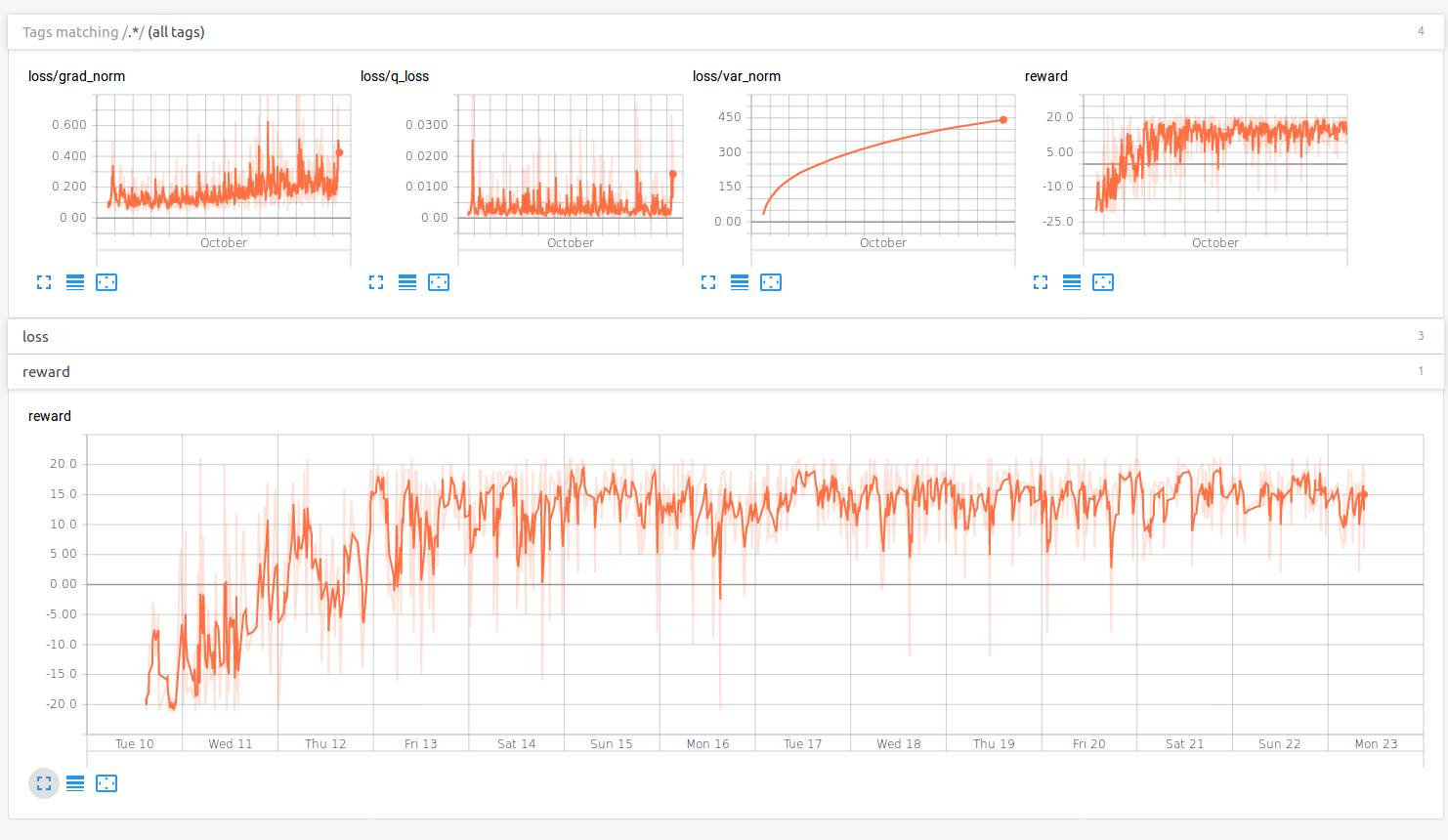
As you can from the above graph, the network was able to consistently win the game after 2 days of training. I haven’t played with exploration parameter of \(\epsilon-\)greedy policy but I think it can be used to improve the performance of the algorithm rapidly especially by introducing a decay.

Dueling network

Dueling network were first introduced in the paper. The core idea in the Dueling networks lies in the following equation:

The above equation says that Q-values can be written as sum of advantage values \(A(s, a)\) and value function \(V(s)\). As it can be seen from the equation, the advantage function tells us the goodness of an action at a state compare to the average total reward at this state \(V(s)\).

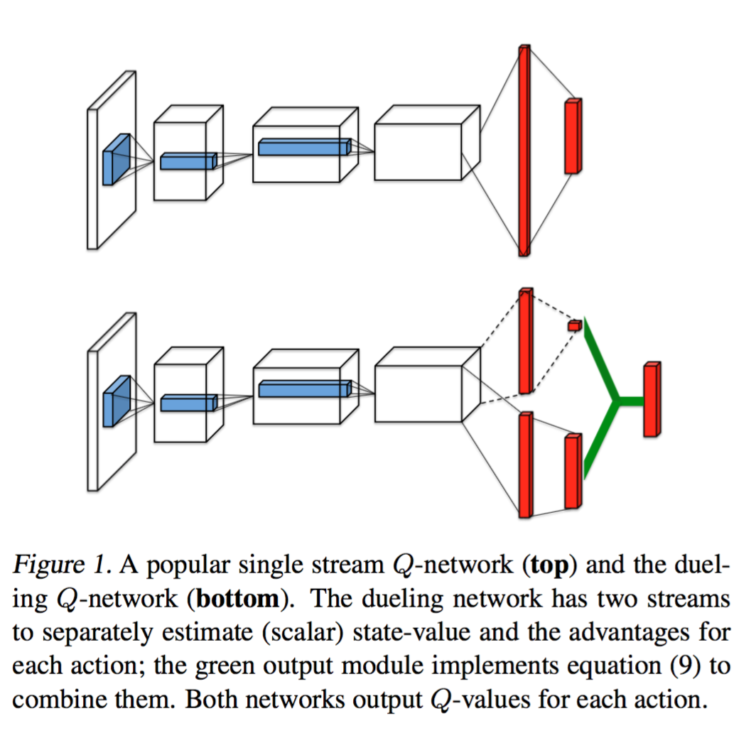
The above paper tells us that instead of computing the Q-values directly, we will compute the advantage \(A(s, a)\) and values \(V(s)\) first and then combine them to get the Q-values. Other than, this architectural change, the rest of the learning process is same as in the Q-learning. This architectural change in the network can be seen in the following figure.

The benefit of doing this architectural change is explained in the following figure in the paper.

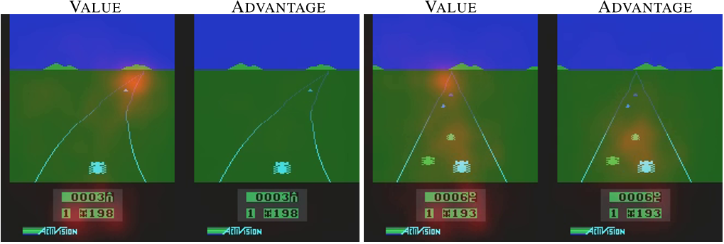
The above figure is the saliency map of a trained model. These maps tell us that the most important pixels that are responsible for high activations in value-function and advantage-function. The left two figures are corresponding to a state where there is no immediate danger to the player and all the actions are safe. In this case, value function is looking at far in the future and focusing on a car that can be a potential threat in future while the saliency map of advantage-function does not show any importance to any pixel. In the right two figures, there are immediate dangers to the agent and the advantage-function learns to focus on those pixels that can cause these immediate danger while value-function is still focusing on the future rewards.

In essence, the above figure tells us that the value network learns to look in far future and the advantage function learns to find the optimal action for the immediate future. By distributing the learning of immediate and future rewards to advantage and value-function respectively, dueling network is known to learn faster. It is also evident in our experiment as shown in the figure below.

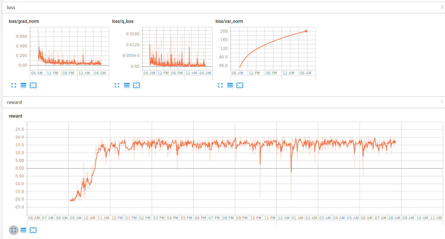
As it can be seen from the above figure, dueling agent learns to play pong effectively within two hours of training.

Moreover, implementing dueling network is also easy. There is only one small detail that we need to take care of. Note that Q-values are the summations of advantage and value function. Note that if we decrease the advantage-function by a constant and increase the state-values by the same constant, we will get the same Q-values. We are training on Bellman error in Q-values and there is no way for us to know the exact advantage and state values and this can cause instability in the learning. To overcome this problem, the authors proposed a solution to put a constraint on Advantage function. The constraint that the authors proposed is that the mean of advantage values for all the actions is zero. With this constraint, the whole model for the Dueling network can be few lines of python code in tensorflow.

def dueling_network(states, is_training=False):
    W1 = tf.get_variable("W1", [state_dim, 20],
                         initializer=tf.random_normal_initializer())
    b1 = tf.get_variable("b1", [20],
                         initializer=tf.constant_initializer(0))
    z1 = tf.matmul(states, W1) + b1
    bn1 = z1
    if use_batch_norm:
        bn1 = batch_norm_wrapper(z1, is_training)
    h1 = tf.nn.relu(bn1)
    W_a = tf.get_variable("W_a", [20, num_actions],
                         initializer=tf.random_normal_initializer())
    b_a = tf.get_variable("b_a", [num_actions],
                         initializer=tf.constant_initializer(0))
    a = tf.matmul(h1, W_a) + b_a
    a = a - tf.reduce_mean(a, axis=1, keep_dims=True)

    W_v = tf.get_variable("W_v", [20, 1],
                        initializer=tf.random_normal_initializer())
    b_v = tf.get_variable("b_v", [1],
                        initializer=tf.constant_initializer(0))

    v = tf.matmul(h1, W_v) + b_v
    q = a + v
    return q